Cournot model
- The Cournot model is built on the following assumptions
- Firms choose the output they will produce, based on the belief of what the other firm is supplying to the market
- The market price is determined by the inverse demand function and the amount supplied by the two firms
- Both firms supply homogeneous goods, and firms have mutual interdependence
- Demand is linear, both firms have a constant marginal cost, and no fixed costs
- This model results in profits above the competitive level, and below the monopoly level (even without collusion)
Example
\[ \begin{aligned} P &= 100- Q \\ MC&=ATC=10 \end{aligned} \]
Suppose each firm believes that the other firm will maintain its current output.
Suppose a duopoly market where there are two firms, Airbus and Boeing. Airbus observes that Boeing currently produces \(q_B=45\), the industry joint profit-maximizing level of output and price is $55. Observing Boeing’s production, how much will Airbus produce?
Airbus takes Boeing’s production into account and calculate the residual demand, represented by the following inverse residual demand curve: \[ P= 100-45-q_A \]
We assume that Airbus’s takes the residual demand that is left over after Boeing has chosen its output level.
Then Airbus will produce \(q_A\), where \(MR_A = MC\). \[ \begin{aligned} MR &= 55-2q_A = MC=10 \\ \therefore q_A &= 22.5 \end{aligned} \]
This means that total industry output is now \[ \begin{aligned} Q &= q_B+q_A = 45 + 22.5 = 67.5 \\ P &= 100-67.5=32.5 \end{aligned} \]
Now Boeing responds to Airbus’s output. If Boeing assumes that Boeing maintains its output at 22.5, then Boeing’s residual demand curve is \[ \begin{aligned} P &= 77.5-q_B \\ MR&=77.5-2q_B = MC =10 \\ \therefore q_B&= 33.75 \end{aligned} \]
This means that total industry output is now \[ \begin{aligned} Q &= q_B+q_A = 33.75 + 22.5 = 56.25 \\ P &= 100-56.25=43.75 \end{aligned} \]
Airbus realizes that Boeing did not maintain its production at 45. According to Cournot model, this game keeps going and Airbus now assume that Boeing will maintain its output at 33.75. Then Airbus’s residual demand curve is \[ \begin{aligned} P &= 100-33.75-q_A = 66.25-q_A \\ MR & = 66.25-2q_A = MC = 10 \\ \therefore q_A&= 28.125 \end{aligned} \]
This means that total industry output is now \[ \begin{aligned} Q &= q_B+q_A = 33.75 + 28.125 = 61.875 \\ P &= 100-61.875=38.125 \end{aligned} \]
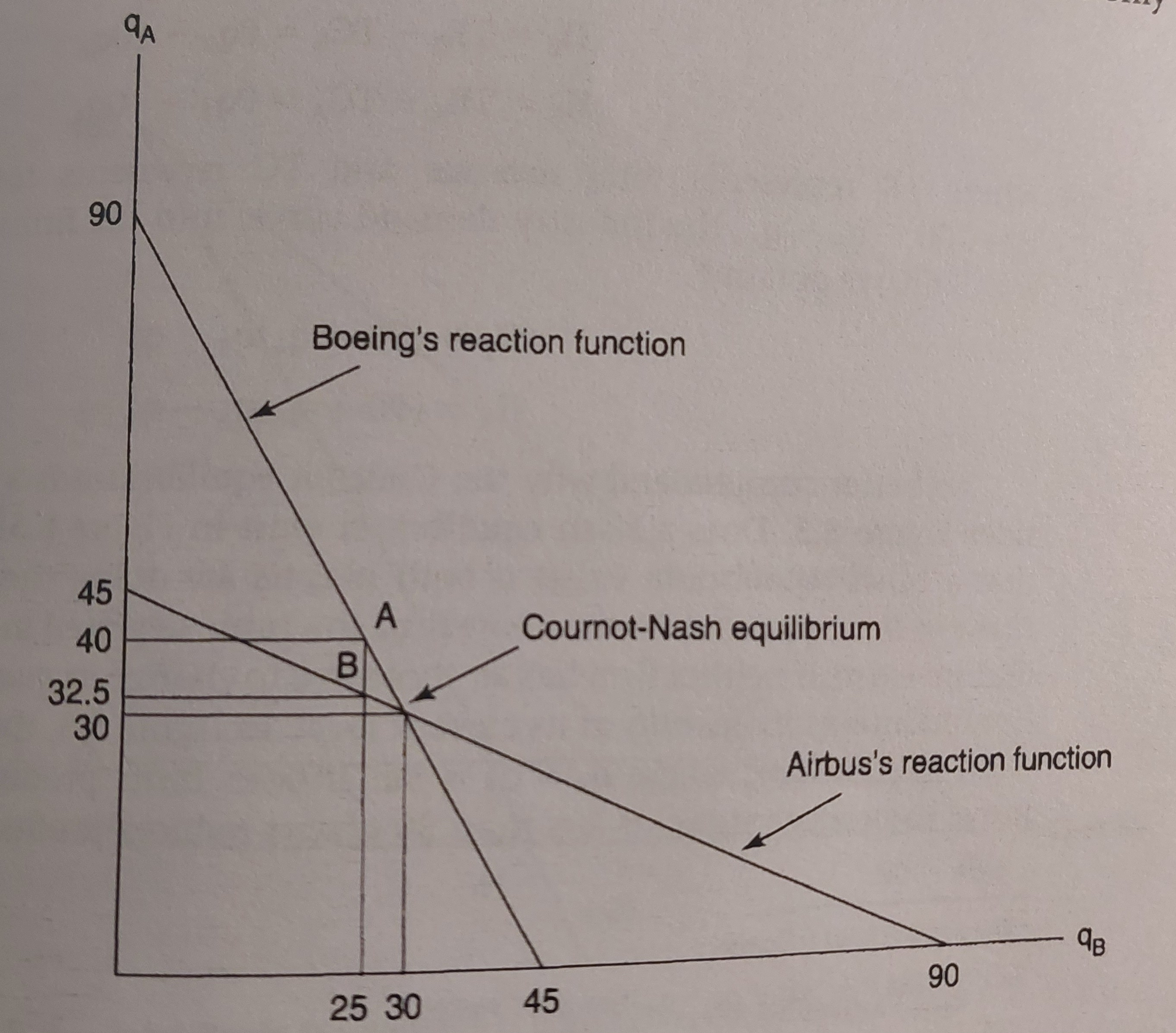
Such adjustment of output continues until both parties correctly anticipated the other player’s output. This happens when Boeing’s reaction function intersects with Airbus’s reaction function. The functional relationship that defines how each party responds to the other party’s output is called reaction function. Boeing’s reaction function and Airbus’s reaction function are respectively represented as follows: \[ \begin{aligned} q_B &=45-\frac{1}{2}q_A \\ q_A &= 45-\frac{1}{2}q_B \end{aligned} \]
This is because each party reacts to the other party’s production to make a decision about it’s optimal output level.
Above reaction functions are derived by solving for profit-maximizing quantity having the other party’s output as given (treat the other party’s quantity constant).
\[ \begin{aligned} TR_B&=q_B(100-q_B-q_A) \\ MR_B&= \frac{\partial TR_B }{\partial q_B} = 100-2q_B - q_A \\ MR_B&=100-2q_B-q_A = MC = 10 \\ q_ B&= \frac{90-q_A}{2} = 45-\frac{1}{2}q_A \end{aligned} \]
Drawing the response functions on the same graph, we have
Another Example
Suppose there are the incumbent and the entrant compete on quantities.
Let’s first start with monopoly and investigate the effect of entry of the equally efficient firm. Assume the inverse demand curve is given by \[ P = 100-0.1Q, \text{ and } \]
the monopolist’s marginal cost and average total cost equals to $40.
Monopolist’s profit
Without new entrant, monopolist produces \[ \begin{aligned} MR_m &= 100-0.2Q = MC = 40 \\ Q_m &=300 \\ P & = 70 \end{aligned} \]
Its profit amounts to \[ \begin{aligned} \Pi_m &= (P - ATC)Q_m \\ &= (70-40)300\\ &= 9000 \end{aligned} \]
Dupolist’s profit in Cournot Model \[ \begin{aligned} P = 100-0.1(q_I + q_E), \end{aligned} \]
where \(q_I\) denotes incumbent’s output and \(q_E\) denotes entrant’s production level.
Setting \(MR_I = MC\) and \(MR_E=MC\), we have
\[ \begin{aligned} 100-0.2q_I -0.1q_E &= 40 \\ q_I &= \frac{60-0.1q_E}{0.2} \\ 100-0.2q_E-0.1q_I &= 40 \\ q_E &= \frac{60-0.1q_I}{0.2} \end{aligned} \]
Solving for system of equations, we have \[ \begin{aligned} q_I &= 200\\ q_E&= 200 \\ P&= 60 \end{aligned} \]
Each firm’s profit amounts to \[ \begin{aligned} \Pi_I &= (P - ATC)Q_I \\ &= (60-40)200\\ &= 4000 \\ \Pi_E &= (P - ATC)Q_I \\ &= (60-40)200\\ &= 4000 \end{aligned} \]