Types of Price Discrimination

Price discrimination is the act of selling the same product at two or more prices
Intuitively, this means charging two different prices for the same good
Mathematically, price discrimination is present if \[ \frac{P_1}{MC_1} \neq \frac{P_2}{MC_2}, \] where the subscripts denote two separate markets, consumers, etc.
Economic definition vs legal definition

First-degree price discrimination (perfect price discrimination)

Assume that a monopolist has perfect information about every consumer
A firm prices the good exactly at each consumer’s willingness to pay

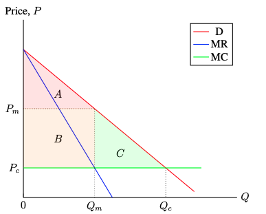
Under perfect competition,
- Consumer surplus = A+B+C
- Producer surplus = 0
Under monopoly,
- Consumer surplus = A
- Producer surplus = B
- Deadweight loss = C

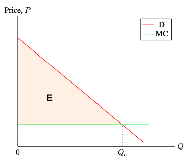
Under perfect price discrimination,
- Consumer surplus = 0
- Producer surplus = E

Second-degree price discrimination

Assume that a monopolist has limited information about consumers about their reservation prices
Second-degree price discrimination is often associated with quantity discounts
All consumers are offered the same price schedule, and they self-select into different price categories

Suppose that Ralph Lauren produces a pair of designer jeans and sell them with quantity discounts.

MC=AC=$20
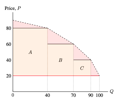
A consumer pays $80, $60, $40, and $20 for the first, the second, the third and the fourth jeans that they buy.
Suppose 10 consumers buy in each of the four price categories
- 10 consumers bought just one pair of jeans
- 10 consumers bought two pairs of jeans
- 10 consumers bought three pairs of jeans
- 10 consumers bought four pairs of jeans
This means that 100 pairs of jeans were sold in total, 40 of them sold at $80, 30 of them sold at $60, 20 of them sold at $40, and 10 of them sold at $20.
In this example,
- Consumer surplus will be the summation of the red shaded regions
- Producer surplus will be 4000 (A+B+C)
However, depending on the price schedule set by the producer, the welfare implication is not clear
- The second degree price discrimination could improve or reduce welfare compared with a uniform price policy

Third-degree price discrimination

Suppose a monopolist sells its output in two separate markets with distinct demand curves
This causes the monopolist to make two decisions in order to maximize profits:
1. How much total output to produce
2. How much of that output to sell in each market
Once these decisions have been made, prices will be set in the two markets according to their respective demands.

Under these conditions, the firm’s total profit is given by \[ \Pi = P_1Q_1+P_2Q_2-TC(Q), \] where $Q=Q_1+Q_2$ To maximize profit, we are solving for the following optimization problem of \[ \max_{Q_1, Q_2} \Pi \] This implies that \[ \begin{aligned} \frac{\partial \Pi}{\partial Q_1} &=MR_1 - MC =0 \\ \frac{\partial \Pi}{\partial Q_2} &=MR_2 - MC =0 \end{aligned} \] With these conditions, we have \[ MR_1= MR_2 = MC \]

We have three separate graphs: market 1, market 2, and the combination of both markets
The marginal revenue curves are summed horizontally to get a MR curve in terms of $(q_1 + q_2)$
It’s important to note that increasing q in either market 1 or 2 will cause an increase in the total MC. Hence, we will optimize in the combined market $(Q^* = q_1^* + q_2^*)$ and determine $q_1$ and $q_2$ after.

Q is determined by the point where $MR_1 = MR_2 = MC$
Markets 1 and 2 produce output their respective marginal revenue is equal to the marginal cost.
The market with less elastic demand is able to charge a higher price → price discrimination
Recall, the more elastic the demand curve, the more consumers are responsive to a change in price

Claim: if a firm price discriminates between two markets, the market with more inelastic demand will necessarily be charged a higher price

Based on the optimal strategy for profit maximizing monopolist, they produce the quantity where $MC=MR$ \[ \begin{aligned} MR&=P\left(1-\frac{1}{|\eta|}\right) \end{aligned} \]
Generalizing our optimality condition to two separate markets, a price-discriminating monopolist sets $MC=MR_1=MR_2$ \[ \begin{aligned} P_1\left(1-\frac{1}{|\eta_1|}\right) = P_2\left(1-\frac{1}{|\eta_2|}\right) \end{aligned} \]

Solving for Optimal Production

A firm with market power in multiple markets where the costs of production are the same is maximizing profits when the following condition holds: \[ MR_1 = MR_2 = MC \]

Suppose a firm holds a monopoly in two separate markets. The distinct inverse-demand functions for both markets are given below: \[ \begin{aligned} P_1 &= 96-3q_1 \\ P_2 &= 64-q_2 \end{aligned} \]

Production for the two separate markets is done from a central location so marginal costs are the same for producing in both markets: \[ MC = 0.5(q_1 + q_2) -16 \]

Assuming the firm is profit-maximizer, what will the output and pricing combinations for the two distinct markets $(q_1^*, q_2^*, P_1^*, P_2^*)$?

Step 1: Find $MR_1$ and $MR_2$ \[ \begin{aligned} MR_1 &= 96-2\cdot 3q_1 = 96-6q_1 \\ MR_2 &= 64-2\cdot1q_2 = 64-2q_2 \end{aligned} \]

Step 2: Set $MR_1=MR_2$ and solve for $q_2$ as an equation for $q_1$ (or vice versa)

\[ \begin{aligned} MR_1 &=MR_2 \\ 96-6q_1 &= 64-2q_2\\ 2q_2 &= 6q_1 - 32 \\ q_2 &= 3q_1 -16 \end{aligned} \]

Step 3: Plug your equation for $q_2$ into the marginal cost function and simplify so it’s in terms of $q_1$

\[ \begin{aligned} MC &= 0.5(q_1+ q_2)-16 \\ &= 0.5(q_1+3q_1 -16) -16 \\ &= 2q_1 -24 \end{aligned} \]

Step 4: Set $MR_1=MC$ and solve for $q_1^*$

\[ \begin{aligned} MR_1 &= MC\\ 96-6q_1&=2q_1-24\\ 8q_1&=120\\ q_1^*&=15 \end{aligned} \]

Step 5: Plug $q_1^*$ into $q_2$ equation we found in step 2 to find $q_2^*$

\[ \begin{aligned} q_2^\ast&=3q_1^\ast -16\\ &= 3\cdot 15 - 16 \\ &=29 \end{aligned} \]

Step 6: Plug $q_1^*$ and $q_2^*$ into inverse-demand functions to find the prices charged in each market

\[ \begin{aligned} P_1^\ast&=96-3q_1^* \\ &= \$51 \\ P_2^\ast&=64-q_2^* \\ &= \$35 \\ \end{aligned} \]

Final Answer:

\[ \begin{aligned} (q_1^\ast, P_1^\ast) &= (15, \$51) \\ (q_2^\ast, P_2^\ast) &= (29, \$35) \\ \end{aligned} \]