Market Power in Practice
- We’ve established some theory, now we can begin to look at how it can be applied in practice
- Market power is a continuous measure, not discrete
- All firms have some level of market power, even if it’s so small we ignore it
- In practice, we tend to define some threshold of market power that is worth caring about
- Graphical example

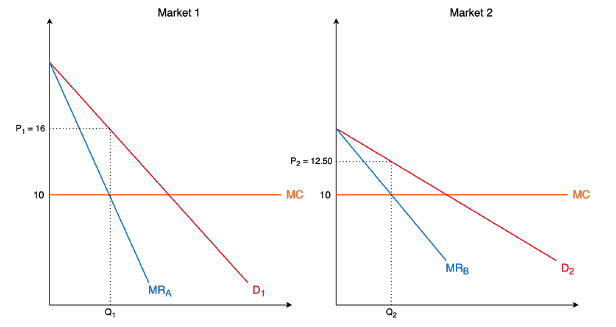
Consider two separate markets where two distinct firms hold a monopoly and face the same constant marginal cost curve.
- The key difference between the two firms is that Firm B faces a more elastic demand curve than Firm A (remember that a flatter curve = more elastic)
Claim: more elastic consumers pay a lower price
- From the graph, we saw that Firm A charges price \(P_1 = \$16\) and Firm B charges price \(P_2= \$12.50\). Additionally, the perfectly competitive price is equal to marginal cost (\(P_c\) = $10) for both firms.
- To prove our claim, first, we can find the Lerner index for both firms to find which firm has more power in the market:
\[ \lambda_1=\frac{P_1-P_C}{P_1} = \frac{16-10}{16}=\frac{3}{8} \]
\[ \lambda_2=\frac{P_2-P_C}{P_2} = \frac{12.5-10}{12.5}=\frac{1}{5} \]
- Next, we can use our simplified equation for the Lerner index to solve for the elasticity of demand for both markets:
\[ \lambda_1=\frac{1}{|\eta_1|} \Rightarrow |\eta_1|=\frac{8}{3} \]
\[ \lambda_1=\frac{1}{|\eta_2|} \Rightarrow |\eta_2|=5 \]
If only one case can be prosecuted, which case would it be?
- Suppose \(Q_c\) where \(D_1=MC\) and \(D_2=MC\) are same across two markets.
- The social welfare loss loss is greater in market 1 than in market 2.
- This means that it may be socially optimal to press charge on firm 1 operating in market 1 if only one case can be prosecuted due to antitrust enforcement cost (each case takes on average 24 months and costs on average $200,000-$250,000).
Excess Profit
Along with Lerner indices, excess profit can be helpful in measuring market power
- Excess profit – firms earning greater return on its resources than necessary
- Excess profit – more entrants into the market
- If we do not observe entrants over time, we expect there to exist some form of barrier to entry (and some degree of market power for the firm enjoying excess profit)
Accounting data is easy to collect; however, this data is not equivalent to economic profit
For the purposes of this class, we will calculate economic profit by including depreciation and opportunity cost
\[ \Pi^e = p\cdot q - TC(q)-D-\gamma \]
- D is economic depreciation of capital stock
- \(\gamma\) is the opportunity cost of the asset (or, in the case of a firm supplying a good, \(\gamma\) is the opportunity cost of producing q units)
- \(D\) and \(\gamma\) are very difficult to measure in practice