Profit Maximization
Under the assumptions previously listed, profit maximization implies that marginal revenue equals marginal cost at the optimal level of production (when \(q = q^\ast\)) \[ MR(q^{\ast}) = MC(q^{\ast}) \]
- Marginal revenue refers to the increase in total revenue when producing an additional unit of output, while it is currently producing \(q\)
- Marginal cost refers to the increase in total cost when producing an additional unit of output, while it is currently producing \(q\)
Intuition
In words, \(MR = MC\) states that profit maximizing firms will continue to scale up production until they can no longer profit from producing an additional unit.
- Thought exercise 1: suppose that marginal revenue is greater than marginal cost
- MR - MC > 0 : can increase profit by producing more
- Thought exercise 2: suppose that marginal revenue is less than marginal cost
- MR - MC < 0 : can increase profit by producing less
Price-taking firms
- The most basic marginal revenue example is a price-taking firm
- A price-taker is an agent that has no control over the market price.
- Consumers are generally price-takers when there are a lot of buyers
- Firms are generally price-takers when there are a lot of competing firms
- If a firm is a price-taker, it means that marginal revenue is equal to the market price \[ MR(q)=p, \, \ \forall q \]
Proit Maximization
- Before finding the profit maximizing level of output, we need to review different cost functions
- Total cost is comprised of fixed costs (costs that remain constant as q increases) and variable costs (costs that increase with additional production).
- Average Cost is the total cost of producing \(q\) units divided by the quantity being produced. \[ AC(q)=\frac{TC(q)}{q} \]
- Average Variable Cost is the total variable cost of producing q units divided by the quantity being produced. \[ AVC(q)=\frac{VC(q)}{q} \]
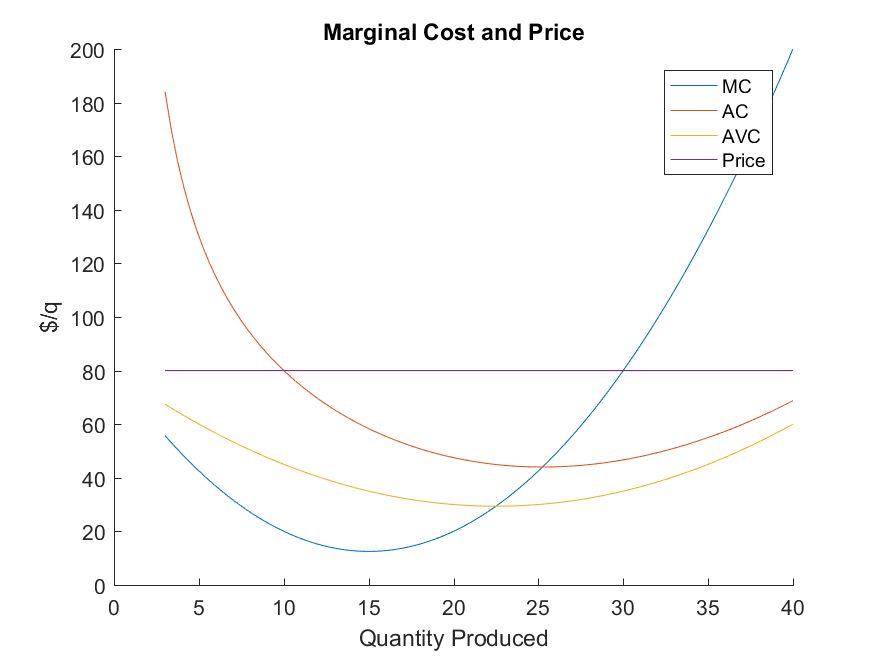
- The market price is $80
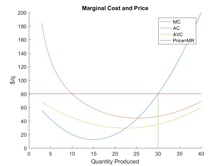
- The profit maximizing point occurs where \(MR = MC\)
- In this example, \(MR = MC\) when \(q^{\ast} = 30\).


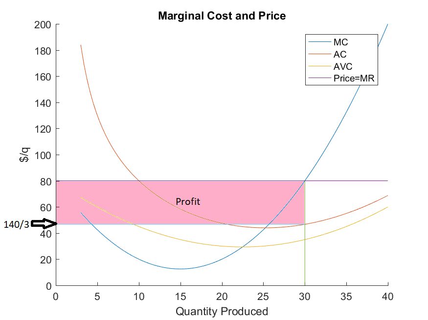
- Profit is shown graphically as the area between price and average cost at the profit maximizing quantity.
\[ \begin{aligned} \Pi(30) &=(p-AC(q^{\ast}))\cdot q^{\ast} \\ &=(80-\frac{140}{3})\cdot 30 \\ &=1000 \end{aligned} \]
Solving profit max problem algebraically
- The graphs were generated using the following total cost function: \[ TC(q)=\frac{1}{10}q^3 - \frac{9}{2}q^2+80q+350 \]
- The associated marginal cost function is given by: \[ MC(q)=\frac{3}{10}q^2-9q+80 \]
\[ \begin{aligned} MC&=MR\\ \frac{3}{10}q^2-9q+80 &=80\\ q \cdot(\frac{3}{10}q - 9)=0\\ q^{\ast}=30 \end{aligned} \]
We can plug in values to find the resulting profit: \[ \Pi(30)= 80 \cdot 30 - (\frac{1}{10}30^3 - \frac{9}{2}\cdot 30^2 + 80 \cdot 30 + 350)=1000 \]